The solver is available here.
I built a linear programming (LP) solver in PyTorch that scales to hundreds of thousands of variables and constraints and is competitive with state-of-the-art solvers on standard benchmark instances. The entire implementation is around 350 lines of core algorithm code, and 600 with documentation and logging. It uses the primal-dual hybrid gradient (PDHG) method (aka the Chambolle-Pock algorithm) -- more specifically, the PDLP algorithm first introduced in the paper Practical Large-Scale Linear Programming using Primal-Dual Hybrid Gradient by Applegate et al (2022). Because the key operations involved are matrix-vector multiplication, building it on PyTorch allows for efficient GPU acceleration. This also allows for support for sparse matrices, which is important for large-scale problems, although PyTorch's sparse support is not yet very mature, so I had to implement some of my own sparse operations. My implementation closely follows the paper cuPDLP.jl: A GPU Implementation of Restarted Primal-Dual Hybrid Gradient for Linear Programming in Julia by Lu et al (2024). However, a bunch of details are not explained in the paper, and the pseudocode is not necessarily written in the way that a programmer would implement it. In this post, I will describe the algorithm along with some additional commentary, discuss some engineering details of my implementation, and lastly show some benchmark results.
We have a linear program of the form: \[ \begin{align} & \text{minimize} \; c^T x \\ & \text{subject to} \\ & Gx \geq h \\ & A x = b \\ & l \leq x \leq u \end{align} \] where \(G \in \mathbb{R}^{m_1 \times n}\), \(h \in \mathbb{R}^{m_1}\), \(A \in \mathbb{R}^{m_2 \times n}\), \(b \in \mathbb{R}^{m_2}\), \(l \in \mathbb{R}^n\), \(u \in \mathbb{R}^n\), and \(c \in \mathbb{R}^n\). We seek to find a vector \(x \in \mathbb{R}^n\) that minimizes the objective function, subject to the constraints.
There are many well-known algorithms for solving LPs, such as the simplex method and interior point methods. However, these methods require expensive matrix factorizations and other linear algebra operations. Instead, PDLP uses a series of matrix-vector multiplications to iteratively update the primal vector \(x\) and a dual vector \(y\). Associated with the above (primal) LP is a dual LP, which maximizes over a vector \(y \in \mathbb{R}^{m_1 + m_2}\) of dual variables. PDLP has seen significant attention recently: the first implementation, to my knowledge, was FirstOrderLp.jl by Google Research. Since then, other implementations have been released such as cuPDLP.jl, COPT's C implementation cuPDLP-C, and it is even now implemented in NVIDIA's cuOPT library.
Sometimes we will want to concatenate the constraints, so we introduce \(K^\top = \begin{bmatrix} G^\top & A^\top \end{bmatrix} \in \mathbb{R}^{(m_1 + m_2) \times n}\) and \(q^\top = \begin{bmatrix} h^\top & b^\top \end{bmatrix} \in \mathbb{R}^{m_1 + m_2}\). Let the sets \(X = \{ x \in \mathbb{R}^n : l \leq x \leq u \}\) and \(Y = \{ y \in \mathbb{R}^{m_1 + m_2} : y_{1:m_1} \geq 0 \}\).
The basic idea of PDLP is to iteratively update \( x, y \) as follows: \[ \begin{align} & x^{k+1} \leftarrow \text{proj}_X(x^k - \frac{\eta}{\omega} (c - K^\top y^k)) \\ & y^{k+1} \leftarrow \text{proj}_Y(y^k + \eta \omega (q - K (2x^{k+1} - x^k))) \end{align} \] where \(\eta \in (0, \infty)\) is the step size and \(\omega \in (0, \infty)\) is the primal weight. PDHG converges for all \( \eta \leq 1 / ||K||_2 \). The projection operator \(\text{proj}\) means to find the point in the set that is closest to the given point. Because of how simple the sets \(X\) and \(Y\) are, the projections are easy to compute: they are essentially just clamping! For \(\text{proj}_X\), we clamp each component of \(x\) to be between \(l\) and \(u\). For \(\text{proj}_Y\), we clamp the first \(m_1\) components of \(y\) to be non-negative.
The papers by Applegate et al (2022) and Lu et al (2024) propose various additions to this basic algorithm, which I recount here in general terms. First, we precondition the matrices in the problem. The step size is adaptive, i.e., not constant. The primal weight is also updated throughout the algorithm. There is also a restart mechanism, where we restart the algorithm from another point in order to help convergence. In the following sections, I will describe each of these additions in more detail, discussing the paper and my implementation.
The preconditioning uses a combination of Ruiz scaling and Pock-Chambolle scaling on the matrix \(K\). Ruiz scaling scales a matrix to have the \(L_\infty\) norm of the rows and columns equal to 1. It is iterative, and theoretically if it is run for infinite iterations, the matrix will achieve that scaling. In practice, we run it for a fixed number of iterations (in my implementation, it is 10). For each iteration of Ruiz scaling, we look at each column of \(K\) and \(c\), and compute a scaling factor as the square root of the maximum absolute value of the column. For each row of \(K\), we look at the maximum absolute value of the row. We then update the problem data as follows:
c, l, u = c / col_rescale, l * col_rescale, u * col_rescale
q = q / row_rescale
K = K * (1.0 / row_rescale).unsqueeze(1) * (1.0 / col_rescale).unsqueeze(0)
constraint_rescaling *= row_rescale
variable_rescaling *= col_rescale
Pock-Chambolle scaling scales a matrix to have the operator norm (which is equivalent to, for the Euclidean norm, the matrix 2-norm, i.e., the largest singular value) less than or equal to 1. The procedure is not iterative like Ruiz, because it is just a matter of constructing the appropriate scaling factors. Again, we look at the rows and columns of \(K\) (note we do not look at \(c\) here), and compute a scaling factor as certain power of the absolute values of the elements. The exponent is mediated by a parameter \(\alpha \in (0, 2)\). We use a default of \(\alpha = 1\), so that the scaling factors are simply the square roots of the sums of the squares of the rows and columns. We then update the problem data and accumulate the scaling factors as above. Throughout the rest of the algorithm, we use the scaled problem data, except for, as we will see, when checking the termination conditions. In order to scale back to the original problem, we simply do:
x_unscaled, y_unscaled = x_scaled / variable_rescaling, y_scaled / constraint_rescaling
The core loop of the algorithm is (taken from Lu et al (2024)):
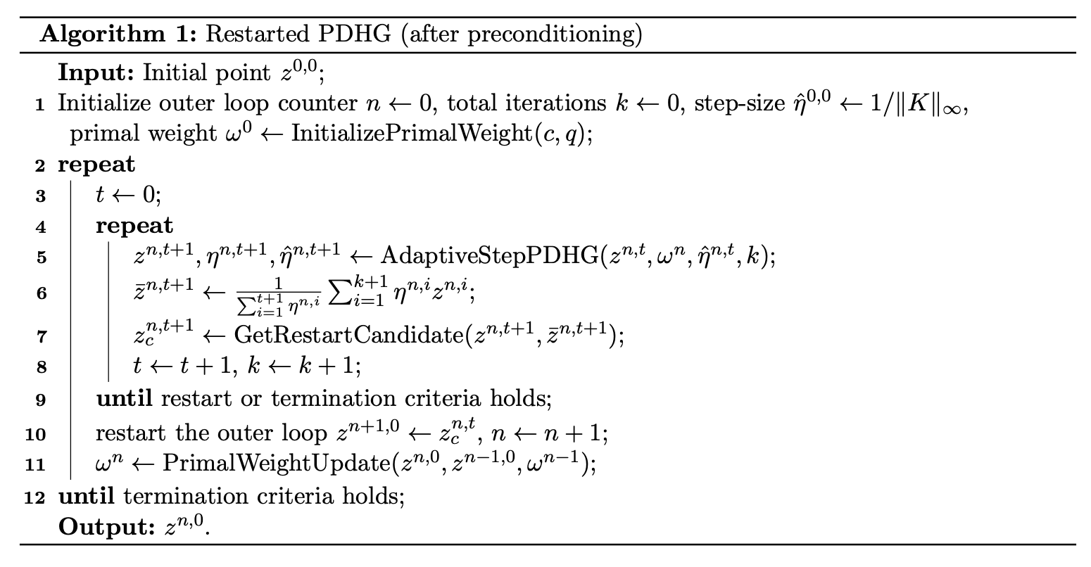
In this algorithm, the inner loop does the actual PDHG steps, i.e., it updates \(x, y\). When a restart condition is triggered, we break out of the inner loop, update the primal weight, and start the inner loop again.
The main confusing thing here are the numerous superscripts. At first glance, this suggests we may need to store a table of variables, over each iteration. However, this is not the case, as we often just need the current or previous iterate. For example, look at line 5. It is simply updating the \(z, \eta, \hat{\eta}\) variables, using the current values of \(z, \omega, \hat{\eta}, k\). What is \(z\)? It is simply the concatenation of \(x\) and \(y\), although in my implementation, I just use \(x\) and \(y\) directly.
In line 6, we are updating a variable \(\bar{z}\) by taking the weighted average of the \(z\) variables, weighted by the \(\eta\) variables -- over their values within this inner loop. I think the summation in this algorithm has an incorrect index: it should be up to \(t+1\), not \(k+1\), as \(t\) is the inner loop counter. Now, we can get around storing every iterate by doing online updating of the weighted averages. We simply need to store the current weighted sum and the current sum of the weights, which can be updated as we go.
In line 7, we get a restart candidate. This function is:
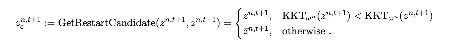
This is just comparing the KKT error of the current iterate \(z\) and the weighted iterate \(\bar{z}\). I will expand on the KKT error in a moment. This function is simple enough that I just do it in-line with a simple if statement.
In line 8 we update counters, and in line 9 we check for the restart or termination conditions. Notably, you should check for termination before checking for a restart! I suppose this is obvious in hindsight, but it is not clear from the pseudocode. In line 10, we update the variables for the next outer loop iteration: the first \(z\) variable for the next loop is set to the restart candidate. In line 11, we update the primal weight.
This is really the crux of the entire algorithm! Take a PDHG step, update the weighted average, and check for restart or termination. Everything can be done online. It admittedly took me a while to wrap my head around this. Because of this, there is actually no need to store the variable \(n\), the outer loop counter, as its sole purpose is to index the variables. We do still need to store \(k\), the total iteration counter, as it is used in the restart criteria, and \(t\), the inner loop counter, as it is used in the PDHG step and the restart criteria. There are a bunch of other details in my implementation, which I will discuss further below. I will now go through each of the subroutines referred to in the main algorithm.
The initial primal weight is set to \( ||c||_2 / ||q||_2 \) if both of these norms are greater than a small nonzero tolerance, otherwise it is set to 1. This is a heuristic: for example, in Applegate et al (2022), they just set it to 1.
This basically implements the PDHG update step, i.e., updating \(x, y\). The main innovation here is the use of an adaptive step size. The algorithm is:
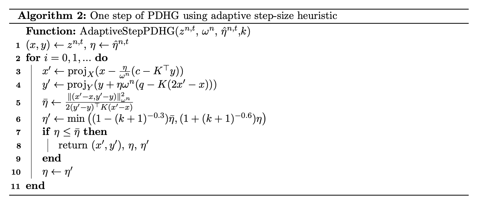
There are a few things going on here. Firstly, \(\bar{\eta}\) is the step size limit. The expression that it is set to in line 5 is a known good bound on the step size for PDHG. So, this algorithm is essentially doing a line search to find a step size that satisfies this good bound. In lines 3 and 4, we compute the new \(x, y\) iterates (recall that the projection is just clamping!). In line 5, we compute the step size limit, and in line 6, we compute a proposal for the next step size, based on a damping of the current step size. We keep doing this until the step size is less than the limit. Then, we return the new iterates, the step size that was used, and the proposed next step size (indeed, refer to the main algorithm to see how these returned values are used).
In line 5, the algorithm uses an operation that looks like \(||z||_{\omega}\) (I omit the superscript on \(\omega\), because it is only important to know that it is the current primal weight). The paper defines \(||z||_{\omega} = \sqrt{\omega ||x||_2^2 + \frac{||y||_2^2}{\omega}}\).
Lastly, I note that there is a missing absolute value: the denominator in line 5 should have an absolute value. This is present in their Julia code, but not in the paper. Indeed, removing this absolute value breaks the algorithm in my testing.
The primal weight update is:
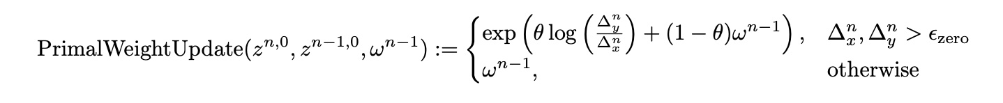
Again, the notation obscures the simplicity of what is going on. You take in the iterate of the current outer loop, the first iterate of the last outer loop, and the current primal weight (note the indices work out like this if you look at where this is called in the main algorithm). You compute the \(L_2\) norm of the difference between the two iterates, and if both are larger than a small non-zero tolerance, you update the primal weight as the exponential moving average of the ratio of these norms and the current primal weight. Note that their formula is missing a \(\log\) on the \(\omega^{n-1}\) (however, this seems to have been corrected in the journal version of the paper).
Lu et al (2024) use the KKT error, as opposed to the normalized duality gap, because the KKT error relies on matrix-vector products, and is hence amenable to GPU acceleration. The KKT error is:
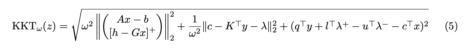
This looks complicated! But it really can just be broken down into a bunch of matrix multiplications. To explain what is going on here, we can write the KKT error as: \[ \text{KKT error}_\omega^z = \sqrt{\omega^2 ||\text{primary residual}||_2^2 + \frac{1}{\omega^2} ||\text{stationarity residual}||_2^2 + (\text{dual gap})^2} \] Note that in my implementation, I do not use the KKT error, but rather the squared KKT error, in order to avoid the square root operation. This also changes the constants used in the restart criteria.
What is this variable \(\lambda\)? It is the dual variable associated with the box constraints, i.e., \(l \leq x \leq u\). This variable lies in a cone at \(x\), defined as: \[ \Lambda = \Lambda_1 \times \Lambda_2 \times \cdots \times \Lambda_n \] where \[ \Lambda_i = \begin{cases} \{0\}, & l_i < x_i < u_i, \\ \mathbb{R}^+, & x_i = l_i, \\ \mathbb{R}^-, & x_i = u_i \\ \end{cases} \] The variable \(\lambda\) is then defined as the projection of \(c - K^\top y\) onto the cone \(\Lambda\). This is easy to compute as we just clamp each component of \(c - K^\top y\) to the appropriate range. Computing the KKT error is intensive, of course. Later, when I expand upon the engineering details of my implementation, I will discuss how to minimize the amount of KKT computations.
The restart criteria is:
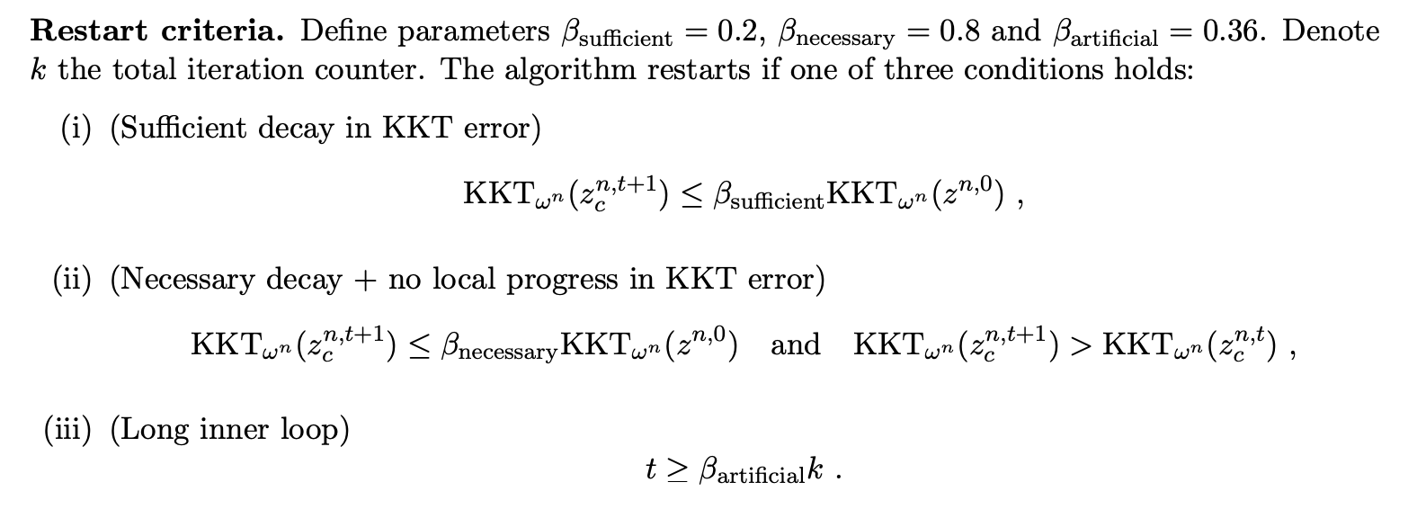
Essentially, if at least one of these three criteria is met, we break out of the inner loop and restart from the restart candidate. The first one says that the KKT of the current candidate is sufficiently smaller than the KKT of the first iterate from the current outer loop. The second says that the candidate has KKT error smaller than the first iterate from the current outer loop and the candidate's KKT is larger than the last candidate's KKT. The third one says that the inner loop counter has exceeded a multiple of the total iteration counter (this is why we need to store both). Each of these criteria are mediated by coefficients that determine the thresholds for the comparisons (the \(\beta\) coefficients). In my implementation, I simply check these conditions in-line with an if statement, at the end of the inner loop. Now, if you followed the previous discussion of how we need not store the history of iterates, you may wonder how we can compute the KKT error of the first iterate of the last outer loop. Indeed, we can simply just compute and store its KKT error in the outer loop, before we enter the inner loop -- we don't need to store the iterate itself. I discuss this in more detail in the implementation details section.
The termination criteria is:
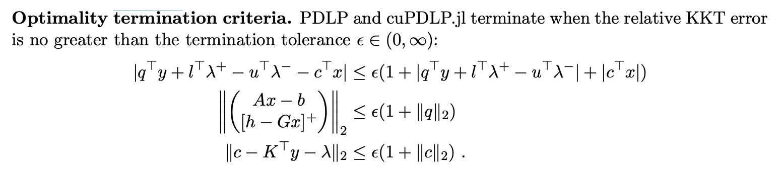
Again, this looks hefty, but is really just a bunch of simple matrix operations. The \(\lambda\) variable is computed as above. Importantly, the conditions are checked against the original unscaled problem data!
The termination conditions above are to check for optimality. But, there are two other possibilities for the problem: it may be infeasible or unbounded. To detect these cases, we rely on a fundamental result from duality theory: the primal is infeasible if and only if the dual is unbounded, and it is unbounded if and only if the dual is infeasible. We can check for infeasibiility by checking for unboundedness of the dual by seeing if the current \(y\) iterate forms a ray (this is called a Farkas certificate). Vice versa, we can check for unboundedness of the primal by testing if the current \(x\) iterate is a ray (which would be a Farkas certificate for the dual).
In this section, I will discuss some of the key engineering details of my implementation. Firstly, I will discuss the online updates of the weighted average, and then the KKT error computation.
As discussed above, we need not store the history of iterates to do line 6 in the main algorithm. We can do this online as follows:
eta_sum += float(eta_used)
alpha = float(eta_used) / eta_sum
x_bar = x_bar + alpha * (x - x_bar)
y_bar = y_bar + alpha * (y - y_bar)
We need to compute the KKT error during two different places in the algorithm: when getting the restart candidate and when checking the restart conditions. To get the restart candidate, we need the KKT of the current iterate and the KKT of the current average iterate. To check the restart conditions, we need the KKT of the current candidate, the last candidate, and the KKT of the first iterate of the current outer loop.
It seems like this requires 5 different KKT computations! However, note that the KKT of the current candidate is simply either the KKT of the current iterate or the average iterate, depending on which one is smaller, so I just assign it as a variable using the same if statement as when we assign the restart candidate. For the KKT of the previous candidate, I simply store this at the end of the inner loop. For the KKT of the first iterate of the current outer loop, I compute this at the top of the outer loop, before we start running PDHG steps inside the inner loop.
Hence, though at first glance it seems like we would need to compute 5 different KKT errors, we actually only need to compute 3, and indeed only 2 in the inner loop. Furthermore, we don't need to store the history of the iterates, we need only compute and store the KKT error in the appropriate place.
In the termination criteria check, the product \(K^\top y_{\text{unscaled}}\) is computed multiple times: namely, it is used when computing the dual objective value and then again when checking the stationarity condition. Hence, we can cache this product at the top of the inner loop, and then reuse it when needed. In my code, I just compute all needed matrix products at the top of the inner loop, and pass them to the functions as needed:
Gx, Ax, KTy = G @ x, A @ x, K.T @ y
x_unscaled, y_unscaled = x / variable_rescaling, y / constraint_rescaling
G_orig_x, A_orig_x, KT_orig_y = G_orig @ x_unscaled, A_orig @ x_unscaled, K_orig.T @ y_unscaled
Gx_bar, Ax_bar, KTy_bar = G @ x_bar, A @ x_bar, K.T @ y_bar
def kkt_error_sq(
    x: torch.Tensor,
    y: torch.Tensor,
    w: torch.Tensor,
    Gx: torch.Tensor | None = None, # cached G @ x
    Ax: torch.Tensor | None = None, # cached A @
    KTy: torch.Tensor | None = None, # cached K.T @ y
) -> torch.Tensor:
We do not check for termination or restarting every inner loop iteration. Instead, we check it every 50 iterations, or every iteration in the first 10. We also only compute a restart candidate in the same loop, as it is only useful if we are actually going to restart. This cuts down significantly on the expensive computations in the KKT calculations and the termination checks. We also check for termination before checking for a restart.
If the termination criteria indicates that the problem is infeasible or unbounded, we ignore this for the first 10 iterations, as these certificates can be false positives in early iterations.
We handle the trivial cases where there are no variables or no constraints before we even start the algorithm, as this will of course cause issues later when trying to, e.g., do matrix multiplications with empty matrices. If there are no variables, we need to check that \(h <= 0\) and \(b = 0\) in order to be feasible. If this is not satisfies, we can construct a certificate of infeasibility. If there are no constraints, then there is an optimum if all variables are bounded in the direction of the objective, otherwise it is unbounded, in which case we can construct a certificate of unboundedness.
The entire implementation is written in PyTorch. All new tensors created are moved to the same device as the problem data. Hence, if the problem data is passed in on the GPU, all computations are done on the GPU. Hence, the entire implementation is GPU-accelerated, as we will see in the benchmarks.
Sparse matrices are essential for large problems. While PyTorch's sparse matrices do not support all operations that are needed for the algorithm, it does support most of them. It supports sparse matrix-vector products, which is what we use throughout the algorithm. We do not use matrix-matrix products, although PyTorch does now support them. Basic arithmetic is supported as well. However, it does not support column maximums nor row maximums, both of which are needed for Ruiz scaling. Also, it does not support slicing, which is needed to reconstruct the matrices \(G\) and \(A\) from the scaled \(K\). Hence, I had to implement my own sparse versions of these operations. For column max/mins, I use the scatter_reduce_ operation, and for slicing, I first coalesce() the sparse matrix, and then obtain the indices and values in order to slice it. Note that I only use COO format for the sparse matrices, as it seems that support for other formats on the GPU is not fully developed (and, e.g., it does not allow some simple operations like transpose)
The solver is available here. The entire implementation is in one file, pdlp.py, and indeed in one function, solve. Just pass your problem data into solve, and it will return the solution.
import torch
from pdlp import solve

# define problem data
c = torch.tensor([1.0, 2.0, 3.0])
A = torch.tensor([[1.0, 0.0, 0.0], [0.0, 1.0, 0.0], [0.0, 0.0, 1.0]])
b = torch.tensor([1.0, 2.0, 3.0])
l = torch.tensor([0.0, 0.0, 0.0])
u = torch.tensor([1.0, 1.0, 1.0])

x = solve(c=c, A=A, b=b, l=l, u=u)
print(x)
There is also a simple CLI, where you can pass problem data from an MPS file. Simply run python pdlp.py problem.mps. The CLI file also contains a function to parse MPS files, so you can import this if you wish to parse MPS files in code.
I benchmarked the solver on a subset of problems from the well-known Mittelman benchmarks of various sizes. You can see the benchmarking file in benchmarks/mittelmann. I ran it on Google Colab. In order to compare CPU and GPU performance, I ran all benchmarks with the tensors on the CPU as well as CUDA. All tensors were made sparse (indeed, I think the problems are too big to be dense). The CPU is an Intel(R) Xeon(R) CPU @ 2.20GHz, and the GPU is an A100 (you can use a T4 for free on Colab). I set a time limit of 1 hour and a tolerance of \(10^{-4}\).
The results are shown in the table below:
| Problem | Rows x Cols | NNZ (% of entries) | GPU Status | GPU Time (s) | CPU Status | CPU Time (s) |
|---|---|---|---|---|---|---|
| qap15 | 6,330 x 22,275 | 94,950 (0.0673%) | Optimal | 10.20 | Optimal | 71.97 |
| a2864 | 22,117 x 200,787 | 20,078,717 (0.4521%) | Optimal | 37.15 | Optimal | 2884.04 |
| ex10 | 69,608 x 17,680 | 1,162,000 (0.0944%) | Optimal | 1.88 | Optimal | 73.35 |
| s82 | 87,878 x 1,690,631 | 7,022,608 (0.0047%) | Time limit | 3600 | Time limit | 3601.68 |
| neos-3025225 | 91,572 x 69,846 | 9,357,951 (0.1463%) | Optimal | 137.18 | Time limit | 3602.36 |
| rmine15 | 358,395 x 42,438 | 879,732 (0.0058%) | Optimal | 57.69 | Optimal | 2396.96 |
| dlr1 | 1,735,470 x 9,142,907 | 18,365,107 (0.0001%) | Time limit | 3601.19 | Time limit | 3600 |
As can be seen, the solver scales well to large problems, especially so on the GPU. Indeed, the GPU provided significant speedups for all problems, going up to 40x for the ex10 benchmark. Comparing the runtimes to the benchmarks on the Mittelmann website, we can see that our solver is competitive with state-of-the-art solvers. For example, the qap15 benchmark is solved in 10.20 seconds on the GPU, while it took HIGHS 22 seconds, GLOP (Google's linear programming solver) 117 seconds, and SoPlex 4022 seconds. For ex10, our runtime is only 1.88 seconds on the GPU, while it took CLP (Coin-OR's linear programming solver) 32 seconds, COPT 1 second, MOSEK 14 seconds, HiGHS 47 seconds, GLOP 479 seconds, SoPlex 296 seconds, and XOPT 2 seconds. Note that these benchmarks are not directly comparable, as, e.g., I don't know what tolerance they used, nor what hardware they used, and I am certain they all used some form of presolve. However, I am still quite pleased that it achieved such runtimes, given the simplicity of the implementation!
One issue I observed is numerical instability in the benchmarks that did not terminate, like dlr1. After analyzing the logs, I found that the duality gap was blowing up, eventually becoming so large that it became nan. I tried various methods to control this, like clamping the step size, but nothing seemed to work. I suppose some solace is that several of the state-of-the-art solvers also did not terminate for dlr1 (with a 250 minute limit).
In this post, I described the PDLP algorithm and its implementation in PyTorch. I went over the pseudocode in detail and then discussed some important implementation details. I benchmarked the solver on a subset of problems from the Mittelman benchmarks, and showed that it scales well to large problems, especially so on the GPU. The algorithm is, in hindsight, quite simple to implement, and I am pleased with its scalability and performance.